Network Capacity Forecasting Before Congestion Bites

Congestion is a forecasting failure, not a bandwidth failure

When a WAN link starts dropping video and stalling backups at 4 p.m. every day, the instinct is to buy a bigger circuit. That fixes the symptom for a quarter or two, then the same wall arrives again — because the real problem was never the size of the pipe. It was that nobody saw the growth curve early enough to act on a purchase-order timeline instead of an emergency one.

Capacity forecasting is the discipline that replaces the fire drill with a boring, scheduled upgrade. It is distinct from sizing a circuit for a known workload: sizing answers "how big should this link be today," while forecasting answers "when will today's link run out, and how confident are we in that date." The difference matters because circuits, transit contracts, and hardware all have lead times measured in weeks, and budgets are approved on annual cycles. A forecast you trust three to six months out is worth more than a perfectly sized link you discover you need next week.

This post covers the method: how to baseline from real telemetry, how to model trend and seasonality, what headroom targets actually protect you, and how to translate a forecast into an upgrade and a budget line.

Baseline from telemetry, not from the vendor's brochure

You cannot forecast a curve you have never measured. Most capacity surprises trace back to organizations planning on nameplate speeds and monthly-average graphs, both of which hide the thing that hurts. Build the baseline from three complementary sources:

• Interface counters via SNMP. Poll every interface for inbound and outbound octets, errors, and discards. This is your ground truth for utilization and the first place congestion shows up as rising output-queue drops.
• Flow telemetry (NetFlow, IPFIX, sFlow). Counters tell you a link is full; flow records tell you what filled it — which applications, which sites, which direction. You cannot forecast demand you cannot attribute.
• Path and quality metrics. Latency, jitter, and loss per path reveal congestion that utilization alone misses, especially on links carrying real-time media.

The single most important modeling choice is what statistic you forecast. Do not forecast the average — averaging a 24-hour day buries the busy hour that breaks experience. Forecast the 95th percentile of the busy period: the level your link sustains most of the time during peak, with brief spikes excluded. The 95th percentile is also how most transit and burstable circuits are billed, so forecasting it aligns your engineering signal with your invoice. Poll at one-to-five minute granularity, roll up to a daily busy-hour p95, and keep at least twelve to eighteen months of history so seasonal patterns become visible.

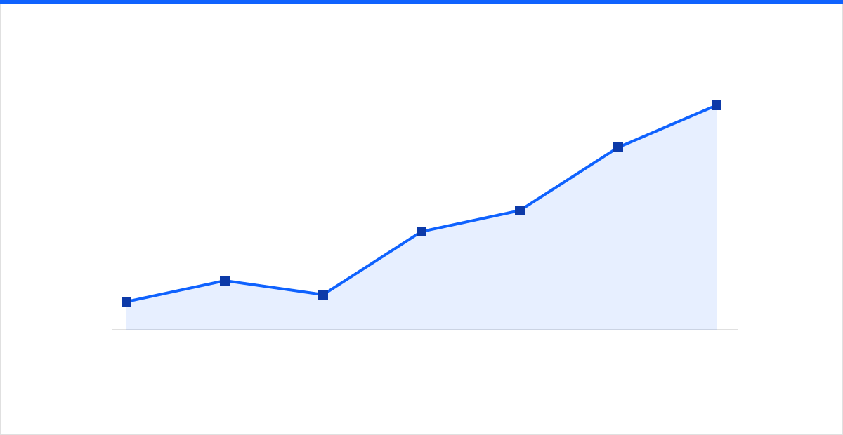Figure: a p95 utilization trend projected forward tells you the exhaustion date months ahead — early enough to buy on a normal procurement cycle, not an emergency one.

Separate the trend from the seasonality

A raw utilization line is the sum of several signals, and forecasting works only after you pull them apart:

• Trend is the slow, underlying climb from more users, heavier applications, and new cloud services. This is what determines your exhaustion date.
• Seasonality is the repeating pattern: daily busy hours, a weekly Monday-morning peak, a monthly close, a quarterly reporting cycle, a retail holiday surge. It rides on top of the trend and is predictable once you have enough history.
• Noise and one-offs are the rest — a one-time data migration, an outage that suppressed traffic, a bad poll. These must be identified and excluded before you fit a trend, or a single anomalous week will bend your entire projection.

Practically, that means: decompose the series, fit the trend on de-seasonalized data (a linear or gentle exponential fit is honest for most enterprise links), then add the seasonal profile back to project the actual peaks you will hit. A link trending at three percent growth per month does not exhaust smoothly — it exhausts on the worst day of its worst seasonal week. Forecast that day, not the annual average. Attributing the trend to specific applications with infrastructure monitoring tells you why the line is climbing, which is what lets you challenge or confirm the forecast.

Headroom targets and the danger of sustained high utilization

A common mistake is treating a link as fine until it hits 100 percent. Long before that, sustained high utilization degrades everything that shares the link. As average load climbs past roughly 70 to 80 percent, queuing delay rises sharply and non-linearly — microbursts that a lightly loaded link would absorb now overflow buffers, and you see jitter and loss on exactly the real-time traffic users notice first. The link reports "up" and the monthly graph looks busy-but-healthy while calls break.

So forecast against a headroom ceiling, not the physical maximum:

• Set a target utilization ceiling per link class. A pragmatic default is planning the busy-hour p95 to stay at or below 70 percent of capacity, leaving room for microbursts, failover, and the gap between your forecast and reality.
• Account for failover load. On resilient designs, one path must carry another's traffic during a failure. If two links normally run at 60 percent, a single failure pushes the survivor to 120 percent — instant congestion. Size and forecast so the post-failover load still fits.
• Define the trigger before you need it. The upgrade trigger is not "the link is full." It is "the forecast shows the busy-hour p95 crossing the headroom ceiling within the procurement lead time." That is the number that goes on the dashboard.

Forecasting growth and the events that break the curve

Steady organic trend is the easy part. The events that cause real outages are the step changes your smooth model will never predict on its own, so fold them in deliberately:

1. Project the organic baseline. Extend the de-seasonalized trend forward and mark where it crosses the headroom ceiling. This is your default exhaustion date.
2. Layer in known step changes. A site merger, a headcount plan, a cloud migration, a new VDI rollout, or consolidating internet breakout through a hub each adds a discrete jump. Model these as additions on top of the trend, dated to the rollout.
3. Reserve for one-off surges. Product launches, seasonal peaks, disaster-recovery test failovers, and large data movements are temporary but real. Decide in advance which you absorb with headroom and which you handle by rate-limiting bulk traffic so it cannot starve interactive flows.
4. Bound the forecast with a range, not a single line. Publish a conservative and an aggressive projection. The honest output of a capacity forecast is a window — "this link exhausts between March and June" — which is precisely what a budget owner needs to decide when to commit money.

Architecture changes the forecast as much as growth does. Moving from backhauled traffic to local internet breakout with SD-WAN can cut private-WAN demand sharply and reset the trend line downward, while centralizing sites onto shared global networks redistributes load in ways a single-link projection will miss. Forecast the design you are moving to, not only the one you have.

Turn the forecast into an upgrade and a budget

A forecast that lives in a monitoring tool changes nothing. The value is realized when it drives a decision on a calendar:

• Rank links by time-to-exhaustion, not by current utilization. A link at 55 percent growing fast may exhaust before one sitting at 80 percent and flat. Triage the portfolio by when, not how full now.
• Work backward from lead time. Add the circuit provisioning window, hardware procurement, and change-window scheduling to set the "commit by" date. Cross the headroom ceiling in the forecast, subtract the lead time, and that is when the purchase order must be signed.
• Attach the forecast to the budget request. A trend chart with a dated exhaustion window and a named business driver — "the p95 crosses 70 percent in Q2, driven by the VDI rollout" — approves far faster than an engineer's assertion that a circuit "feels slow."
• Re-forecast every month and close the loop. Compare last month's projection to what actually happened, and adjust. Forecasting is a rolling practice, not an annual spreadsheet, and its accuracy compounds the longer you run it.

Get ahead of the curve

Congestion almost never arrives without warning — the warning simply sits unread in telemetry nobody is trending. Baseline the busy-hour p95 from SNMP and flow data, separate trend from seasonality, forecast against a headroom ceiling instead of the physical maximum, and layer in the step changes and one-off events that smooth models miss. Do that, and the next upgrade becomes a scheduled line item with a defensible date rather than an emergency after users complain.

intSignal baselines, monitors, and forecasts client networks so capacity decisions land on a procurement timeline, not a crisis one. Talk to our network team to turn your telemetry into a forecast you can budget against.