Demand Forecasting With Machine Learning: A Practical Primer

When simple forecasting stops being enough

A surprising amount of the world still forecasts demand with a moving average and a gut check, and for a stable, single product that is often the right call. If a series has a steady level, mild seasonality, and no external drivers, a naive "last week repeats" or an exponential-smoothing model is cheap, transparent, and hard to beat. The mistake is assuming that because a simple method is enough for one series, it is enough for the whole business.

Machine learning starts to pull ahead in three specific situations, and they tend to arrive together:

• Multiple interacting drivers. Demand that responds to price, promotions, weather, holidays, competitor activity, and macro trends has more structure than a smoother can capture. A moving average sees only the past values of the series itself; it is blind to the 30-percent-off promotion that starts Monday.
• Many series at once. Forecasting one item is a statistics problem. Forecasting fifty thousand SKUs across two hundred locations is a scale problem. A single ML model can learn patterns across series — new products borrow the seasonality of similar established ones, and slow sellers inherit signal from the category — which per-series classical models cannot do.
• Nonlinearity and thresholds. Real demand has kinks: a price elasticity that changes above a point, a promotion whose lift saturates, a heat wave that only matters past a temperature. Linear and additive models struggle with these; tree-based and neural models handle them natively.

If none of those apply, do not reach for ML. If two or three do, simple methods are leaving accuracy — and inventory dollars — on the table.

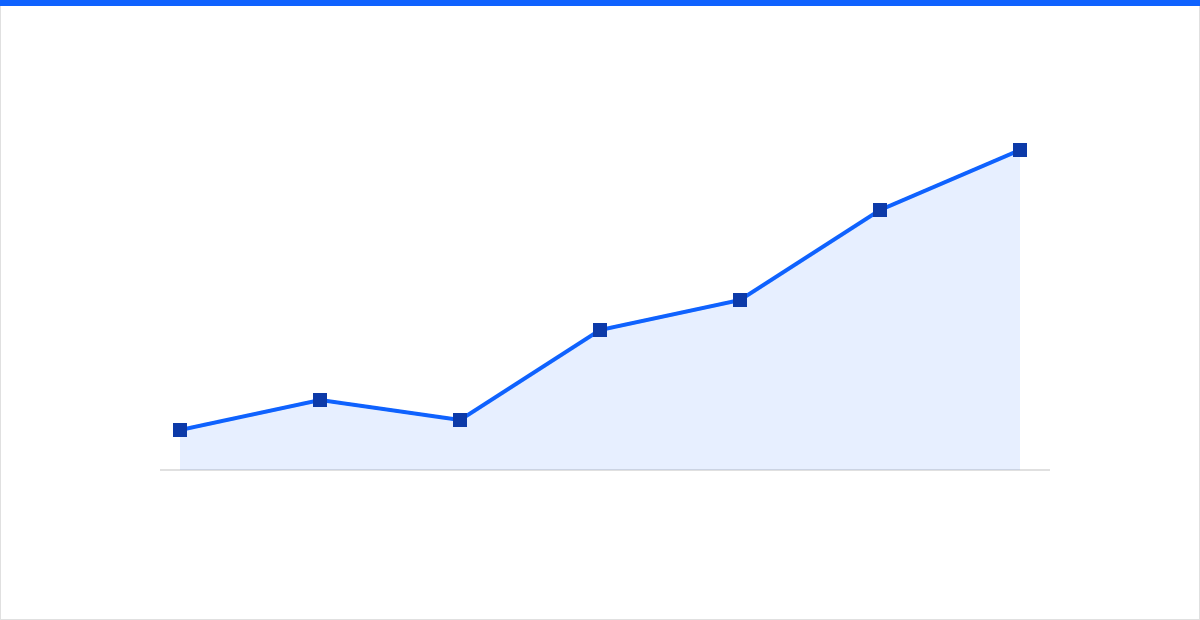Figure: a moving average smooths through the very events — promotions, seasonal peaks — that a driver-aware model is built to anticipate.

Classical, ML, and deep learning: matching method to problem

There is no single best forecaster. There is a best method for the shape of your data, the number of series, and the drivers you need to model. Our machine learning and AI practice treats the choice as a spectrum, not a religion.

Classical statistical methods

Exponential smoothing (ETS) and ARIMA remain excellent for a modest number of series with clear trend and seasonality and few external drivers. They are fast, interpretable, and give calibrated uncertainty for free. They are the right default for a new program and the baseline every fancier model must beat. Their ceiling: they model each series in isolation and struggle to absorb many external regressors.

Gradient-boosted trees

For most business forecasting at scale, gradient-boosted decision trees are the workhorse and frequently the winner. You reframe forecasting as a supervised regression problem — engineer features from the history and the calendar, then predict the next value — and train one global model across all series. Trees handle nonlinearity, ignore irrelevant features gracefully, and train on millions of rows quickly. This is where a large share of real-world programs land.

Deep learning

Neural approaches earn their complexity when you have very long histories, many related series, or rich covariates that reward learned representations. They can also produce full probability distributions directly. The cost is real: more data, more tuning, more compute, and less transparency. Reserve them for problems where tree-based models have plateaued and the volume justifies the overhead. The cloud infrastructure to train and re-train them on a schedule is usually the easy part; the data discipline around them is not.

Features are where accuracy is actually won

Across every method above, the single biggest lever is not the algorithm — it is the features you feed it. A well-fed gradient-boosted model beats a poorly-fed neural network almost every time. The feature set that consistently pays off:

• Calendar and seasonality. Day of week, week of year, month, and payday cycles. Encode holidays explicitly, and encode the days around them — the pull-forward before Thanksgiving and the dead week after matter as much as the day itself.
• Promotions and price. Discount depth, promo type, display and feature flags, and the relative price versus the usual shelf price. Promotions are often the largest source of variance and the hardest for naive methods to see.
• Lags and rolling windows. The value 1, 7, and 28 days back; rolling means and standard deviations over trailing windows. These give the model recent level and volatility without hand-tuning a smoother.
• Weather. Temperature, precipitation, and severe-weather flags drive demand for a huge range of categories, from beverages to generators to HVAC parts.
• Product and location context. Category, brand, region, store format, and demographics let a global model share signal across similar series and cold-start new items sensibly.

Building and maintaining this feature set reliably is a data-engineering job as much as a modeling one, and it is where a data analytics foundation quietly determines whether the whole program works.

Evaluating a forecast honestly

Forecasting is unusually easy to fool yourself on, because a model that looks great in a random split can be worthless in production. Two disciplines keep you honest.

Backtest the way time actually moves. Never use a random train/test split for a time series — it lets the model peek at the future. Use rolling-origin evaluation (also called walk-forward): train on data up to a cutoff, forecast the next horizon, roll the cutoff forward, and repeat. This simulates exactly how the model will be used and exposes seasonality it has not yet seen.

Pick error metrics that match the decision. Report more than one:

• MAPE (mean absolute percentage error) is intuitive but explodes on low-volume or intermittent items and cannot handle zeros — a single near-zero actual can dominate the average.
• WAPE (weighted absolute percentage error) aggregates absolute error and divides by total demand, so high-volume items get proportional weight. For most inventory decisions it is the more honest number.
• Bias — the signed error — matters as much as magnitude. A model that is 10 percent off but always high is a very different (and more expensive) problem than one that is 10 percent off in both directions, because persistent over-forecast quietly inflates inventory.

Always compare against the naive baseline. If your ML model cannot beat "last season repeats," it is not ready, and the honest move is to keep the simple method.

Forecast intervals, because a point is not a decision

A single predicted number is nearly useless for planning, because the whole point of a forecast is to size a buffer against being wrong. What inventory, staffing, and capacity decisions actually need is a range: the model should say the 90th percentile of demand is a certain level, and you stock to the service level your economics justify. The gap between the point forecast and that upper quantile is your safety stock, and it should be wider for volatile items and narrower for predictable ones. Quantile forecasting — predicting the distribution rather than the mean — is what turns a model output into a defensible ordering policy. A team that only ships point forecasts has done half the job.

Pitfalls that quietly wreck a model

• Data leakage. The classic killer: a feature that would not be known at prediction time sneaks into training — using a promotion flag set after the fact, or a target that is transformed using future values. Leakage produces gorgeous backtest numbers and a model that collapses in production. Audit every feature for "could I actually know this when I forecast?"
• Overfitting. A model tuned until it memorizes the noise in your history looks brilliant on the past and generalizes poorly. Rolling-origin validation, honest holdouts, and a bias toward simpler models are the defenses.
• Ignoring intermittent demand. Slow-moving items with many zero-demand periods break percentage metrics and mislead standard models. They need methods built for intermittency, not a one-size-fits-all pipeline.
• Set-and-forget. Demand patterns drift as products, prices, and behavior change. A model that is never retrained decays silently. Monitor its live error the way you monitor a service, and retrain on a schedule.

Get the forecast to earn its keep

Machine learning demand forecasting is not about the flashiest model. It is about matching the method to your data, feeding it the drivers that actually move demand, backtesting the way time really flows, and shipping intervals a planner can decide against. Done that way, it compresses both stockouts and overstock at the same time — the same win predictive analytics delivers everywhere it is done well. intSignal builds and runs these pipelines as a managed capability, from machine learning and AI strategy through the data plumbing and the retraining loops that keep accuracy from decaying. If your planning still runs on spreadsheets and gut feel, talk to our team and we will find the first series where a better forecast pays for itself.