Anomaly Detection: The Techniques Behind the Alerts

Why a fixed line is the wrong tool

Every monitoring platform ships with the same starting point: a static threshold. Alert when CPU crosses 90 percent, when latency passes 500 milliseconds, when the error rate exceeds 1 percent. It is simple, explainable, and wrong often enough to be expensive. A threshold that is quiet at 3 a.m. is deafening at the Monday morning login surge. A threshold tuned for the busy tier pages constantly on the idle one. Set it loose and you miss slow degradations; set it tight and you drown the on-call in false alarms until they mute the channel.

The core problem is that a fixed line has no memory and no context. It does not know that this metric always doubles at month-end close, that Fridays run 30 percent hotter than Tuesdays, or that a value which is alarming for one host is routine for its neighbor. Anomaly detection is the family of techniques that replace the fixed line with a learned notion of normal — one that adapts to time of day, day of week, and the specific behavior of each signal. This post walks through those techniques, from the statistics that solve most cases to the machine learning you reach for when they do not, and the tuning decisions that determine whether the result earns trust or joins the muted channels.

Statistical baselines: distributions, not lines

Before any machine learning, most anomaly detection worth doing is statistics applied carefully. The shift is from a single threshold to a distribution of expected values, updated continuously.

• Rolling z-score. Compute a moving mean and standard deviation over a trailing window, then flag points that sit more than, say, three standard deviations from the mean. This adapts as the metric drifts and needs no labeled data. Its weakness is that a few large spikes inflate the standard deviation and hide the next one.
• Median and MAD. Swapping mean and standard deviation for the median and the median absolute deviation makes the same idea robust to outliers, because a single huge value no longer drags the center. For noisy operational metrics this is often the better default.
• Seasonal decomposition. Real infrastructure signals have structure: a trend, a repeating daily and weekly seasonality, and a residual. Techniques such as STL (seasonal-trend decomposition using loess) split the series into those three parts, then look for anomalies only in the residual — the piece left after you remove the expected shape. This is what catches the Tuesday that looks nothing like every other Tuesday, without firing during the normal evening peak.

The practical rule: if the metric is a well-behaved time series with clear daily and weekly rhythm, seasonal decomposition on the residual solves a large majority of real cases, cheaply and transparently. Reach past it only when the data defeats it.

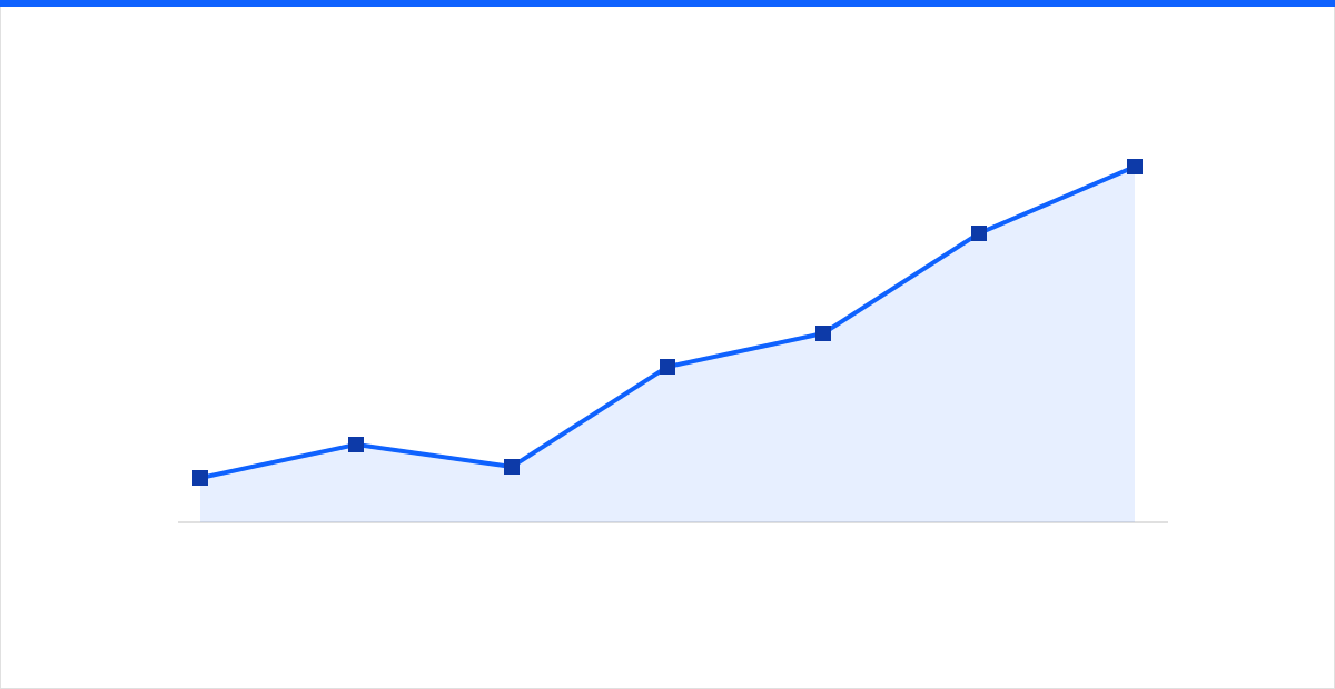Figure: a learned baseline tracks the daily and weekly rhythm, so only the deviation from expected shape — not the normal evening peak — trips an alert.

When statistics are not enough: machine learning

Statistical methods assume you are watching one metric at a time and that its normal shape is describable. Two situations break that assumption: many metrics that are only anomalous in combination, and signals with no clean seasonal shape. Two workhorse models cover most of this ground.

• Isolation forest. Instead of modeling normal and measuring distance from it, an isolation forest exploits a simple fact: anomalies are few and different, so they are easy to separate. The algorithm builds random trees that split the data; points that get isolated in very few splits are, by definition, unusual. It is fast, handles many features at once, needs no labels, and works well for multivariate detection — for example, CPU, memory, disk I/O, and request rate that are each individually normal but jointly impossible.
• Autoencoders. A neural network is trained to compress a signal and reconstruct it. Trained only on normal data, it reconstructs normal patterns accurately and fails on ones it never saw, so a high reconstruction error is the anomaly score. Autoencoders shine on high-dimensional and complex inputs — the shape of a full request trace, a window of log-derived features, or correlated metrics across a fleet — where the normal manifold is too intricate to write down by hand.

Both are unsupervised, which is the point: you almost never have a labeled catalog of anomalies, so the model learns the shape of normal and scores how far each new observation departs from it. The cost is interpretability. A z-score breach explains itself; a reconstruction error of 0.42 does not. Feed model output into machine learning and AI workflows that attach context — which features drove the score, what the metric was doing around it — so a responder can act on the flag instead of second-guessing it.

The precision and recall tradeoff

No detector is free of errors, and the choice of which errors to tolerate is the most consequential decision in the whole exercise. Two numbers frame it:

• Precision — of the things you alerted on, how many were real.
• Recall — of the real anomalies, how many you caught.

They trade against each other. Loosen the model to catch everything (high recall) and you flood the queue with false positives (low precision). Tighten it to alert only when certain (high precision) and you miss the subtle early signals (low recall). There is no universally correct point on that curve — it depends on the cost of a miss versus the cost of a false alarm.

That cost is not symmetric across domains. For a security signal where a missed intrusion is catastrophic, you accept lower precision and more analyst review to protect recall. For a capacity metric where a false page wakes someone for nothing, you favor precision. The failure mode to fear is quiet erosion: a noisy detector trains people to ignore it, so effective recall collapses to near zero regardless of what the model can technically catch. Alert fatigue is not a side effect of bad detection — it is the mechanism by which good detection stops working. Tune to the precision the on-call can sustain, then raise recall only as fast as you can keep the false-positive rate bearable.

Labeling and feedback close the loop

Unsupervised detection gets you started without labels, but it should not stay label-free. Every alert an engineer dispositions — real incident, known-benign, maintenance window, duplicate — is a label you did not have to pay for, and those labels are what turn a static model into an improving one.

1. Capture the disposition, not just the alert. Log why an anomaly was dismissed, so recurring benign patterns can be learned and suppressed rather than re-flagged.
2. Feed confirmed anomalies back as positive examples. Over time this lets a supervised layer sit on top of the unsupervised detector, sharpening precision on the cases you have actually seen.
3. Watch for drift and retrain on a schedule. A migration, a new release, or a traffic pattern shift changes what normal means. A model trained on last quarter's environment quietly degrades; monitor its own hit rate the way you monitor a service, and retrain before it decays.

Without this loop the detector is a depreciating asset. With it, tomorrow's model is built from today's judgment calls.

Metrics, logs, and security use the same core

The techniques generalize once you frame each domain as a signal with a normal shape.

• Metrics. Time-series methods — seasonal decomposition, robust z-scores, multivariate isolation forests — fit directly onto the telemetry a mature infrastructure monitoring practice already collects. The main work is per-metric seasonality, not new math.
• Logs. Logs are not numeric, so the first step is turning them into features: cluster millions of lines into a few dozen templates, then track the rate of each template. A pattern that never existed before, or a known one that spikes, becomes a numeric anomaly you can score with the same tools.
• Security. User and entity behavior — login times, data volumes, access paths — is exactly the kind of high-dimensional signal autoencoders and isolation forests handle well. Piped into a SIEM and reviewed inside a security operations center, behavioral anomaly detection surfaces the compromised account that never trips a signature.

Getting it right

Good anomaly detection is less about the fanciest model than about matching the technique to the signal, choosing a precision the team can live with, and wiring in the feedback that keeps it honest. Start statistical, escalate to machine learning only where the data demands it, and treat every dismissed alert as training data rather than noise. intSignal designs, tunes, and operates detection across metrics, logs, and security telemetry as a managed capability — including the unglamorous work of seasonality, thresholds, and feedback loops that decides whether alerts get trusted or muted. If your monitoring is loud and your confidence is low, talk to our team and we will help you build detection worth acting on.